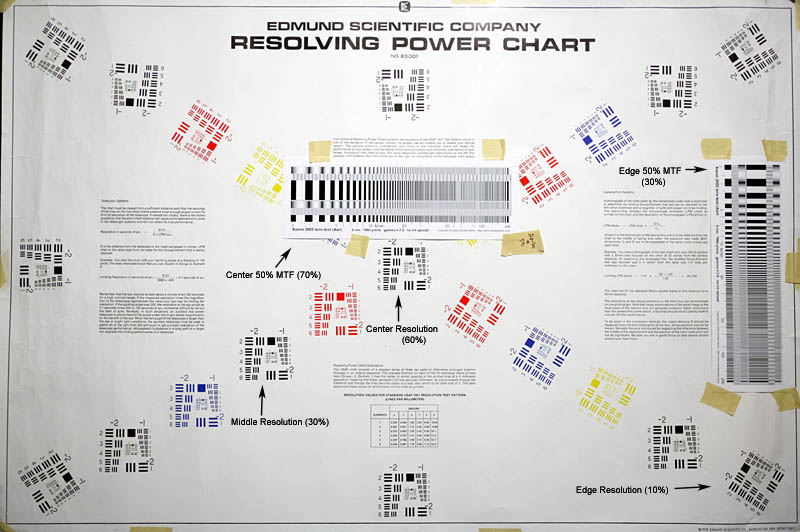
2. The chart is photographed at a working distance that is 1/2 the recommended distance so that the entire Edmund Scientific chart can be photographed for resolution and determination of 50% MTF. It is also possible to detect lateral chromatic and other aberrations from the same test images. The distance from the chart was calculated at d1=(M+1)f where d1 = lens to target distance (mm) and f = lens focal length (mm) and M=25. The reduction of distance by 1/2 requires that lp/mm figures read off the chart be adjusted by 1/2.
3. Photographic RAW files are converted to tifs with Capture One Pro. The tif files are opened in image analysis software to analyze the sine patterns on the chart (top band). I used ImageJ software, public domain software off the NIH site.
Click on "File" and then "Open" to select and open the tif of interest.
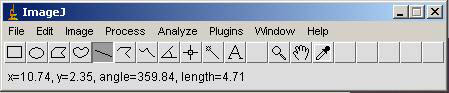
4. Click on the "magnifying cursor symbol" to fill the window with the Koren chart image and click on the "hand" icon to move the chart image into the middle of the window.
5. Click on the line icon and draw a straight line through the upper sine pattern bar on the Koren chart.
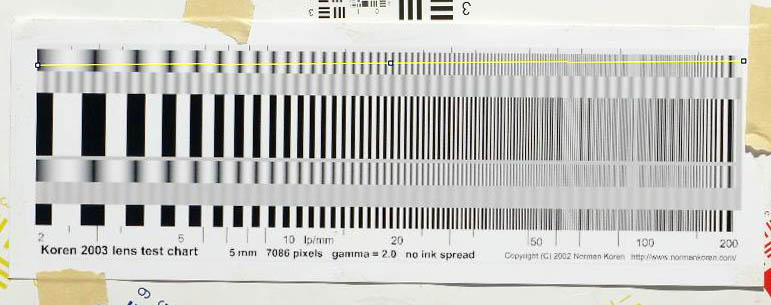
6. Click on the "Analyze" menu and select "set scale" and enter "known distance" as "25" and "units" as "cm".
7. Click on "Analyze" again and select "Plot Profile."
8. A sine wave pattern will be generated and displayed.
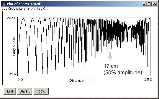
9. The full amplitude of the sine wave on my computer screen has a 7 cm sweep. I just take a rule and run it down the plot towards 25cm until the amplitude is 50% (3.5 cm). In the example, 50% amplitude is at 17 cm on the chart. This corresponds on a plot of cm of chart versus a log plot of spatial frequency below to 147 lp/mm.
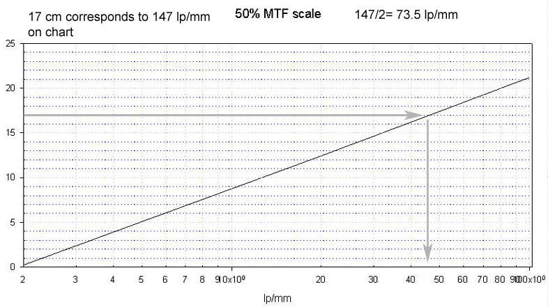
10. Because the working distance was decreased by 1/2 when photographing the chart, the lp/mm value is divided by 2 to generate the 50% MTF value.